Simulation of Most Permissive Boolean networks#
The module mpbn.simulation implements random walks into the Most Permissive (MP) dynamics of a given Boolean networks, for estimating the stationnary distribution.
The method is described in the paper Variable-Depth Simulation of Most Permissive Boolean Networks by Roncalli et al. (2022). The random walk is performed from a given initial configurations and transition probabilies are computed according to two parameters:
the permissivity depth of the transition, where depth 1 corresponds to asynchronous transitions, and further depth characterize the transitions that require permissive interpretation of transitions.
the numer of components that change of value in one transition. The parametrization allow scaling the probability of the transition as a function of these two quantities.
This notebook demonstrates how to use to employ the mpbn.simulation module. Alternatively, the simulations can be performed using the command line utility mpbn-sim. See mpbn-sim --help for usage, and bnediction/mpbn for examples of configuration files (e.g., simulation_bladder.json and simulation_i3ffl2.json files).
Simulations are performed with estimate_reachable_attractors_probabilities and parallel_estimate_reachable_attractors_probabilities functions. These functions require
a Boolean network
f, being either ampbn.MPBooleanNetworkobject or any object supported by its constructor (e.g.,colomini.minibn.BooleanNetworkobject, Python dictionnary, filename in BoolNet format, GINsim or bioLQM objects)an initial configuration
x, being a dictionnary associating components to a Boolean valuea list
Aof attractors reachable fromx, as obtained withf.attractors(reachable_from=init)provided thatfis ampbn.MPBooleanNetworkobjecta number
nb_simsof trajectories to simulatea function
depth()which is called at each simulation step to determine the maximum permissivity depth of transitions to considera vector
Wofnreals (wherenis the number of components off) for determining the rate of a transition in function of the number of components that change of value.
The simulation returns a dictionnary associating the index of the attrarctor in A with its estimated stationnary probability.
The function for the depth parameter can be generated using:
constant_maximum_depth(f): consider all MP transitions for the BNfconstant_unitary_depth(f): consider only (general) asynchronous transitions offpoly_depth(f, power=1.2): random depth with polynomially decreasing probability: if \(n\) is the number of components off: it will draw a maximum depth \(d\) with probability proportional to \((n-d-1)^{power}\)reciprocal_depth(f): draw a maximum depth \(d\) with probability proportional to \(1/d\)nexponential_depth(f, base=2): draw a maximum depth \(d\) with probability proportional tobase\(^{-d+1}\)
The function for the rate parameter can be generated using:
uniform_rates(f): constant uniform ratefully_asynchronous_rates(f): assigns a rate of 1 for transition changing exactly one components, and 0 otherwisereciprocal_rates(f): assigns a rate of \(1/k\) for a transition changing the value of \(k\) componentsnexponential_rates(f, base=2): assigns a rate ofbase\(^{-k-1}\) for a transition changing the value of \(k\) components
import mpbn
import mpbn.simulation as mpsim
from colomoto_jupyter import tabulate # for pretty display
Simple model#
Let us consider the following simple Boolean network we define with mpbn.MPBooleanNetwork:
f = mpbn.MPBooleanNetwork({
    "a": 1,
    "b": "a",
    "c": "(!a & b)|c"
})
f
a <- 1
b <- a
c <- c|(!a&b)
Its full most permissive dynamics from the configuration 000 is the following:
x = f.zero()
x
{'a': 0, 'b': 0, 'c': 0}
f.dynamics(init=x)
# computing graph layout...

its fully asynchronous dynamics is the following:
f.dynamics("asynchronous", init=x)
# computing graph layout...

Thus, we can deduce that the MP transition 000 -> 101 has requires a permissive depth strictly greater than 1 (see the method paper for details).
The simulation functions requires as input the list of reachable attractors. These can be obtained as follows (two fixed point in this example):
A = list(f.attractors(reachable_from=x))
A.sort(key=lambda a: [a[i] for i in f]) # stable ordering, for notebook reproducibility only
tabulate(A)
| a | b | c | |
|---|---|---|---|
| 0 | 1 | 1 | 0 |
| 1 | 1 | 1 | 1 |
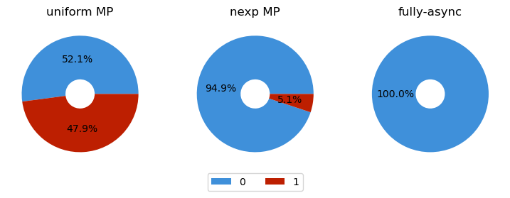
We first estimate their propability in the stationnary distribution from 1,000 simulations of a unform random walk in the full MP dynamics from x:
nb_sims = int(1e3)
urw = mpsim.estimate_reachable_attractors_probabilities(f, x, A, nb_sims,
                        depth = mpsim.constant_maximum_depth(f), # full MP dynamics
                        W = mpsim.uniform_rates(f)) # uniform random walk
urw
100%|███████████████████████████████████████████████████████████████| 1000/1000 [00:00<00:00, 7634.96it/s]
{0: 52.1, 1: 47.9}
Let us compare with exponentially decreasing depth and rate…
edw = mpsim.estimate_reachable_attractors_probabilities(f, x, A, nb_sims,
                        depth = mpsim.nexponential_depth(f),
                        W = mpsim.nexponential_rates(f))
edw
100%|███████████████████████████████████████████████████████████████| 1000/1000 [00:00<00:00, 4209.22it/s]
{0: 94.9, 1: 5.1}
… and considering only fully-asynchronous transitions:
faw = mpsim.estimate_reachable_attractors_probabilities(f, x, A, nb_sims,
                        depth = mpsim.constant_unitary_depth(f),
                        W = mpsim.fully_asynchronous_rates(f))
faw
100%|███████████████████████████████████████████████████████████████| 1000/1000 [00:00<00:00, 6010.25it/s]
{0: 100.0, 1: 0.0}
import matplotlib.pyplot as plt

def make_pie(probs, ax=plt):
    labels=[n for n in names if probs.get(n,0) > 0]
    patches, _, _ = ax.pie([probs[n] for n in names if probs.get(n,0) > 0],
                wedgeprops=dict(width=.75),
                colors=[colors[n] for n in names if probs.get(n,0) > 0],
                autopct=lambda pct: f"{pct:.1f}%")
    return dict(zip(labels, patches))
def make_plot(results):
    nb_cols = len(list(results))
    nb_rows = 1
    fig, axes = plt.subplots(nb_rows, nb_cols, figsize=(3*nb_cols, 3*nb_rows))
    patches = {}
    for col, (label, p) in enumerate(results):
        ax = axes[col]
        patches.update(make_pie(p, ax))
        ax.set_title(label)

    axes[1].legend(patches.values(), patches.keys(),
                            bbox_to_anchor=(0.5, -0.2), # Legend position
                            loc='lower center',
                            ncol=2,
                            fancybox=True)
names = [0,1]
colors = ["#3f90da",  "#bd1f01"]
make_plot([
    ("uniform MP", urw),
    ("nexp MP", edw),
    ("fully-async", faw)])
Larger scale model#
We demonstrate how to import a model in GINsim format and perform simulations in different mutation conditions.
import ginsim
wt_model = ginsim.load("http://ginsim.org/sites/default/files/SuppMat_Model_Master_Model.zginml")
ginsim.show(wt_model)

We convert the model to an mpbn.MPBooleanNetwork object and define its initial state according to the original publications (all nodes but microRNAs inactives, and DNA damage and ECMicroenv active.
f = mpbn.MPBooleanNetwork(wt_model)
init_active = ["miR200", "miR203", "miR34", "DNAdamage", "ECMicroenv"]
x = {node: node in init_active for node in f}
nb_sims = int(1e3)
We compute the reachable attractors from the initial state. The first two attractors correspond to apoptosis while the latter to metastasis.
A = list(f.attractors(reachable_from=x))
A.sort(key=lambda a: [a[i] for i in f]) # stable ordering, for notebook reproducibility only
tabulate(A)
| AKT1 | AKT2 | Apoptosis | CDH1 | CDH2 | CTNNB1 | CellCycleArrest | DKK1 | DNAdamage | ECMicroenv | EMT | ERK | GF | Invasion | Metastasis | Migration | NICD | SMAD | SNAI1 | SNAI2 | TGFbeta | TWIST1 | VIM | ZEB1 | ZEB2 | miR200 | miR203 | miR34 | p21 | p53 | p63 | p73 | |
|---|---|---|---|---|---|---|---|---|---|---|---|---|---|---|---|---|---|---|---|---|---|---|---|---|---|---|---|---|---|---|---|---|
| 0 | 0 | 0 | 1 | 1 | 0 | 0 | 1 | 0 | 1 | 1 | 0 | 0 | 0 | 0 | 0 | 0 | 0 | 0 | 0 | 0 | 1 | 0 | 0 | 0 | 0 | 1 | 0 | 0 | 1 | 0 | 1 | 1 |
| 1 | 0 | 0 | 1 | 1 | 0 | 0 | 1 | 0 | 1 | 1 | 0 | 0 | 0 | 0 | 0 | 0 | 0 | 0 | 0 | 0 | 1 | 0 | 0 | 0 | 0 | 1 | 1 | 0 | 1 | 1 | 0 | 0 |
| 2 | 0 | 1 | 0 | 0 | 1 | 0 | 1 | 1 | 1 | 1 | 1 | 1 | 1 | 1 | 1 | 1 | 1 | 1 | 1 | 1 | 1 | 1 | 1 | 1 | 1 | 0 | 0 | 0 | 0 | 0 | 0 | 0 |
We perform parallel simulations with the specified number of parallel jobs.
mp_wt = mpsim.parallel_estimate_reachable_attractors_probabilities(f, x, A, nb_sims,
                        depth = mpsim.nexponential_depth(f),
                        W = mpsim.nexponential_rates(f), nb_jobs=8)
mp_wt
100%|█████████████████████████████████████████████████████████████████| 1000/1000 [00:25<00:00, 39.98it/s]
{0: 28.8, 1: 51.0, 2: 20.2}
Now, we apply a mutation (p53 loss of function):
f_ko = f.copy()
f_ko["p53"] = 0
We compute the reachable attractors…
A_ko = list(f_ko.attractors(reachable_from=x))
A_ko.sort(key=lambda a: [a[i] for i in f]) # stable ordering, for notebook reproducibility only
tabulate(A_ko)
| AKT1 | AKT2 | Apoptosis | CDH1 | CDH2 | CTNNB1 | CellCycleArrest | DKK1 | DNAdamage | ECMicroenv | EMT | ERK | GF | Invasion | Metastasis | Migration | NICD | SMAD | SNAI1 | SNAI2 | TGFbeta | TWIST1 | VIM | ZEB1 | ZEB2 | miR200 | miR203 | miR34 | p21 | p53 | p63 | p73 | |
|---|---|---|---|---|---|---|---|---|---|---|---|---|---|---|---|---|---|---|---|---|---|---|---|---|---|---|---|---|---|---|---|---|
| 0 | 0 | 0 | 1 | 1 | 0 | 0 | 1 | 0 | 1 | 1 | 0 | 0 | 0 | 0 | 0 | 0 | 0 | 0 | 0 | 0 | 1 | 0 | 0 | 0 | 0 | 1 | 0 | 0 | 1 | 0 | 1 | 1 |
| 1 | 0 | 1 | 0 | 0 | 1 | 0 | 1 | 1 | 1 | 1 | 1 | 1 | 1 | 1 | 1 | 1 | 1 | 1 | 1 | 1 | 1 | 1 | 1 | 1 | 1 | 0 | 0 | 0 | 0 | 0 | 0 | 0 |
… in this example, they are a subset of the attractors reachable in the wild type model:
[a in A for a in A_ko]
[True, True]
We perform simulations on the mutated model giving the wild type attractors for make comparison easier.
mp_KO = mpsim.parallel_estimate_reachable_attractors_probabilities(f_ko, x, A, nb_sims,
                        depth = mpsim.nexponential_depth(f),
                        W = mpsim.nexponential_rates(f), nb_jobs=8)
mp_KO
100%|█████████████████████████████████████████████████████████████████| 1000/1000 [00:19<00:00, 51.08it/s]
{0: 60.0, 1: 0.0, 2: 40.0}
We observe that the mutation substantially increases the probability of the metastasis attractor.